Plotting rasters in R

load required packages

library(raster)      # raster data
library(rasterVis)   # raster data visualisation
library(rgee)        # Google Earth Engine in R
library(sf)          # spatial data handling
library(tidyverse)   # general data wrangling and visualisation

Getting Landcover data from Google Earth Engine

## load the package rgee
library(rgee)

## initialize google earth engine in R
ee_Initialize(drive = T)

## define a region of interest
roi <- ee$Geometry$Rectangle(76.8100, 30.6676, 77.0010, 30.8084)

## load and clip ESA WorldCover 2020 data
landcover2020 <- ee$ImageCollection("ESA/WorldCover/v100")$
  # select the first image
  first()$
  # clip to region of interest
  clip(roi)

## Move results from Earth Engine to Drive
task_img <- ee_image_to_drive(
  image = landcover2020,
  folder = "rgee_backup",
  fileFormat = "GEO_TIFF",
  region = roi,
  fileNamePrefix = "landcover_2020"
)

task_img$start()
ee_monitoring(task_img)

## Move results from Drive to local
img <- ee_drive_to_local(task = task_img, dsn = "data/lc2020.tif")

## deauthorise google drive
googledrive::drive_deauth()

## remove all variables from environment
rm(list = ls())

base R

mwls_lc <- raster("data/lc2020.tif")
plot(mwls_lc)

lattice levelplot

library(raster)
library(rasterVis)

## data from ESA WorldCover 2020 
mwls_lc <- raster("data/lc2020.tif")

levels(mwls_lc) <- data.frame(
    ID = c(seq(10, 60, 10), 80),
    landcover = c("Trees", "Shrubland", "Grassland", "Cropland", "Built-up", 
             "Barren/Sparse \n Vegetation", "Open water")
    )

levelplot(mwls_lc, att='landcover',
          col.regions = c("#006400", "#FFBB22", "#FFFF4C", "#F096FF", "#FA0000", 
                          "#B4B4B4", "#0064C8"),
          colorkey = list(height = 1, labels = list(cex = 1.2)))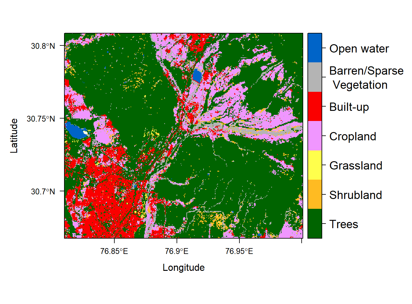

ggplot

## data from ESA WorldCover 2020 
mwls_lc <- raster("data/lc2020.tif")

## a function to convert raster to dataframe
rasterdf <- function(x, aggregate = 1){
    resampleFactor <- aggregate
    inputRaster <- x    
    inCols <- ncol(inputRaster)
    inRows <- nrow(inputRaster)
    
    # Compute numbers of columns and rows in the new raster for mapping
    resampledRaster <- raster(ncol = (inCols / resampleFactor),
                              nrow = (inRows / resampleFactor))
    
    # Match to the extent of the original raster
    extent(resampledRaster) <- extent(inputRaster)
   
    # Resample data on the new raster
    y <- resample(inputRaster, resampledRaster, method='ngb')
   
    # Extract cell coordinates  
    coords <- xyFromCell(y, seq_len(ncell(y)))
    dat <- stack(as.data.frame(getValues(y)))
    
    # Add names - 'value' for data, 'variable' to indicate different raster layers
    # in a stack
    names(dat) <- c('value', 'variable')
    dat <- cbind(coords, dat)
    dat
}

## convert raster to data frame
mwls_df <- rasterdf(mwls_lc)

## prepare legend
LCcodes <- c(seq(10, 90, 10), 95, 100)
LCnames <- c("Trees", "Shrubland", "Grassland", "Cropland", "Built-up", 
             "Barren/Sparse Vegetation", "Snow and Ice", "Open water",
             "Herbaceous wetland", "Mangroves", "Moss and lichen")
LCcolors <- attr(mwls_lc, "legend")@colortable[LCcodes + 1]
names(LCcolors) <- as.character(LCcodes)

## plot the map
ggplot(data = mwls_df) +
  geom_raster(aes(x = x, y = y, fill = as.character(value))) + 
  scale_fill_manual(name = "Land cover",
                    values = LCcolors[-c(7, 9:11)],
                    labels = LCnames[-c(7, 9:11)],
                    na.translate = FALSE) +
  coord_sf(expand = F) +
  theme(axis.title.x = element_blank(),
        axis.title.y = element_blank(),
        panel.background = element_rect(fill = "white", color = "black"))

## remove all variables from the environment
rm(list = ls())